Machine learning models

1
2
3
4
5

# install required packages
pip install numpy
pip install tensorflow-cpu
import numpy as np
import tensorflow as tf

Linear regression

\(\hat {y} = z = w^T . x + b\)

1

%timeit np.dot([[0.5, 0.5]], [1, 0]) + 0.2 # 0.7

1

%timeit tf.matmul([[0.5, 0.5]], [[1], [0]]) + 0.2

Logistic regression

\(\hat {y} = a = \sigma(z)\)

Activation funtions

• Linear funtion \(a = z\)

For predicting real number at the output layer.

• Sigmoid \(\sigma = a = \frac{1}{1+e^{-z}}\) - For Binary classification, Output in range [0, 1].
• Tanh = \(\frac {e^z - e^{-z}} {e^z + e^{-z}}\) - Mean at 0, Output in range [-1, 1].
• Relu = $max(z, 0) $
• LeakyRelu = $max(z, 0.1*z) $
• Softmax = \(\frac {e^z} {\sum_{i=1}^{n} e^z_i}\)
  • Used for multi-class classification.
  • If class 2, its same as logistic regression.
  • Loss function \[l(\hat{y}, y) = - \sum_{j=1}^c y_j log (\hat{y}_j)\]
• Hardmax takes the max value in vector and sets it to 1, the rest will to 0.

1

 np.exp(1)

Note: e = Euler’s number ~= 2.718

 1
 2
 3
 4
 5
 6
 7
 8
 9
10

def activation(z, grad=False):
    """ Sigmoid activation funtion.
    """
    a = 1/ (1 + np.exp(-z))
    return a

def forward(W, B, X):
    Z = np.dot(W, X.T) + B
    A = activation(Z) # where A is Y^
    return A

 1
 2
 3
 4
 5
 6
 7
 8
 9
10
11
12
13
14
15
16
17
18
19
20
21
22
23
24
25

def visualize(X, Y, A, epoch=None):
    """Helper funtion to monitor the models prediction/loss.
    """
    if epoch is not None:
        error = np.mean(loss(Y, A))
        print(f"@epoch {e}, {error=:4f}")
    else:
        print("-------------------")
        print("Input| Y | Y^")
        print("-----|---|---------")
        for i, gt, p in zip(X, Y, A.ravel()):
            print(f"{i}| {gt} | {p:4f}")
        print("-"*19)

X = np.array([[0, 0],
              [0, 1],
              [1, 0],
              [1, 1]])
Y = np.array([0, 0, 0, 1])

W, B = np.array([[0.0, 0.0]]), 0.0
#W, B = np.array([[0.5, 1]]), 0.2

A = forward(W, B, X)
visualize(X, Y, A)

Objective funtion

• Logistic loss \(L(\hat{y}, y) = - ({y \log \hat y + (1-y)\log( 1- \hat y)})\)

  • must be a convex funtion

• Cost funtion \(J = \frac {1} {m} \sum_{i=1}^m {L(a^i, y)}\)

1
2
3
4

def loss(y, y_hat):
    """Loss funtion to help calculate the error during the training process.
    """
    return -(y* np.log(y_hat) + (1-y)* np.log(1-y_hat))

Gradient decent

$w := w - α × \frac{dj(w)} {dw} $

• Learning rate = \(\alpha\)

• Momentum

• Derivation = slop = \(\frac {hight} {width}\)

  • For as small change in width what is th change in hight?
  • At different instance of the funtion. the derivation will change. It is not be constant.
  • Eg 1)

  \[ f(a) = a^2 , df(a)/da = 2a \\ df(a)/da, a = 2 ; 4 \\ df(a)/da, a = 5 ; 10 \]

  • Eg 2)

  \[ f(a) = log(a); df(a)/da = 1/a \\ df(a)/da, @ a = 2; 0.5 \]

  • For multiple varible (chain rule)

    \[f(a,b,c) = 3(a + bc)\] Reducing the above funtion; \[ j = 3v \\ v = a + u \\ u = b * c\\ \] Now to finding the derivation \[ dj/dv = 3 \\ dj/du = dj/dv * dv/du = 3 * 1 = 3 \\ d(j)/da = dj/dv * dv/da = 3 * 1 = 3 \\ d(j)/db = dj/dv * dv/du * du/db = 3 * 1 * c = 3c \\ d(j)/dc = dj/dv * dv/du * du/dc = 3 * 1 * b = 3b \]

Lets place the puzzles together;

1. For differentiation of J with respect to a;

\[j = - y log(a) + (1-y) log( 1- a) \\ dj/da = - y/a + 1-y/1-a \]

1. For differentiation of a (activation funtion) with respect to z;

\[ a = 1/(1+e^-z) \\ da/dz = a(1-a) \]

Reference https://towardsdatascience.com/derivative-of-the-sigmoid-function-536880cf918e

1. For differentiation of J with respect to z;

\[ dj/dz = dj/da * da/dz \\ = - (y/a + 1-y/ 1-a) * a (1 - a)\\ = -y +ya + a -ya\\ = a - y\\ \]

1. For differentiation of z with respect to w and b;

\[ z = w.x+b\\ dz/dw = x\\ dz/db = 1\\ \]

1. Finally the gradients we are after

differentiation of J with respect to w and b. \[ dj/dw = dj/da * da/dz * dz/dw\\ dj/dw = x (a - y)\\ \\ dj/db = dj/da * da/dz * dz/db\\ dj/db = (a - y) \]

Gradient for different activation

\[ {sigmod}(z) = dg(z)/dz = a * (1-a) \\ {tanh}(z) = dg(z)/dz = 1 - a^2\\ {relu}(z) = dg(z)/dz = 0 if z< 0 ; 1 if z>=0 \\ {leaky\_relu} = dg(z)/dz = 0.1 if z< 0 ; 1 if z>=0 \]

 1
 2
 3
 4
 5
 6
 7
 8
 9
10
11

def backward(A, Y, X):
    # - (y/a + 1-y/ 1-a) * a (1 - a)
    dZ = A - Y
    dW =  X.T * dZ # (2, 4) (number of features, number of input examples) * (4 , 1) (number of input examples, 1)
#    dW =  np.dot(X , dZ) # (2, 4) (number of features, number of input examples) * (4 , 1) (number of input examples, 1)
    dB = dZ

    dW = np.mean(dW) # (2, 4) (number of features, number of input examples)
    dB = np.mean(dB)
    #keepdims=True, axis=1
    return dW, dB

 1
 2
 3
 4
 5
 6
 7
 8
 9
10
11
12
13
14
15
16
17
18
19
20
21
22

epoch = 100
learning_rate = 1

X = np.array([[0, 0],
              [0, 1],
              [1, 0],
              [1, 1]])
Y = np.array([0, 0, 0, 1])

W, B = np.array([[0.0, 0.0]]), 0.0
for e in range(0, epoch):
    A = forward(W, B, X)
    dW, dB = backward(A, Y, X)

    if e % 9 == 0:
        visualize(X, Y, A, epoch=e)

    W -= learning_rate * dW
    B -= learning_rate * dB

visualize(X, Y, A)
print(f"{W=}, {B=}")

Neural networks

Weight update

\[ dz_2 = a_2 -y\\ dw_2 = dz_2 . a_1.T\\ db_2 = dz_2\\ \\ z_2 = w_2.T z_1\\ dz_1 = W_2.T . dz_2 * (dg/dz_1)\\ dw_1 = dz_1 . x.T\\ db_1 = dz_1\\ \]

Initialization of weights

W and b are set to a small random value.

1
2
3
4

number_of_units, number_of_input_nodes = 2, 2
w = np.random.randn(
    (number_of_units, number_of_input_nodes)) * 0.01
b = np.zeros((number_of_units,1))

• Setting \(W^{[1]}\) = [[00] [00]] will make \(a^1_1 = a^1_2\);

ie both the nodes will be learning the same funtion (same dz during the weights updates)

• Setting the constant 0.01 will ensure the values are lower and if larger values are set as W then the activation funtion will be at the higher end; where the gradent will be close to 0 (no learning will happen).

• Although in practice \(\sqrt{\frac 2 {n^{[l-1]}}}\) will be used as constant to minimize the vanishing/exploding gradients (where the gradients get too big or too small during training and lead to hight bias).

  • where n is the number of features and the variance of the weight will be \(\frac 2 n\) for relu activation or \(\frac 1 n\) for tanh activation or in some cases $\frac 2 {n[l-1] + n[n]} $.
  • The intution here is the higher the number of input features smaller the weights one expects to be initialized.

Regularization

Notation: \(\lambda\) is the regularization parameter.

1. L1 regularization cost funtion =

\[ J = \frac {1} {m} \sum{}_{i=1}^m L(\hat {y}, y) + \boxed{\frac \lambda {2m} ||w||_1^1} \\ \]

• where w will be sparse (for compressing the model, with weights pushed to 0).

• L2 regularization

cost funtion = \[J = \frac {1} {m} \sum{}_{i=1}^m L(\hat {y}, y) + \boxed{\frac \lambda {2m} ||w||_2^2}\]

• where \(||w||_2^2 = {\sum{}_{j=1}^n w_j^2} = {w^T w}\) is the square euclidean norm of weight vector w.

• During gradient decent; \(w = w - \alpha \frac {dj}{dw}\) and \(\frac {dj}{dw} = x \frac {dj}{dz} + \boxed{\frac \lambda {m} w^{[l]}}\)

  • The weight decay here is;

\[ w[l] = w[l] -\alpha [ \frac {dj}{dw} + \frac \lambda {m} w[l]] \\ w[l] = w[l] - \frac {\alpha \lambda}{m} w[l] - \alpha \frac {dj}{dw}\\ w[l] = \boxed{(1 - \frac {\alpha \lambda}{m}) w[l]} - \alpha \frac {dj}{dw}\\ \]

by forcing the weights to a smaller range, the output of activation funtion will facilate

• mostly linear funtion (a simpler model)
• the gradient to be higher during training.
• Dropout

Randomly turn off the nodes during training; will force different nodes to learn from different features and not overfit.

• During training (inverted dropout is the technique used here)and during inference there is not dropout.

 1
 2
 3
 4
 5
 6
 7
 8
 9
10
11
12

# mimicking activation output from layer x.
a = np.array([0.4, 0.5, 0.9, 0.1])

# probability of keeping the node.
keep_probability = 0.5

drop_out_layer = np.random.rand(
                                        a.shape[0],
                                        a.shape[1]) < keep_probability
a = np.multiply(a, drop_out_layer)
# scaling by the keep probability
a /= keep_probability

> this will help with the test time (without having to implementation dropout). > else this scaling factor will be added into the test time (which only adds to more complexity).

• If the dropout is used in the first layer of the neural network the input features will be randomly turned off forcing the model to spead its weights to learn more robustly similar to \(L_2\) regularization.

• The cost function will not show the errors going down smoothly, since we are killing of the nodes in random.

• Early stopping

Save the model which performs best of the validation set, and stop the training where there is no further improvements on validation set after x number of epochs.

Orthogonalization

• minimizing the cost funtion
• avoiding overfitting

Preprocessing

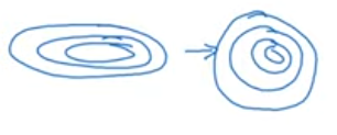
Normalizing your input will change the shape of the search space in a favarable manner (makes the training more efficient).

• Normalizing

x - min / max - min

\[\mu = \frac 1 {m} \sum_{i}^m X^{(i)} \\ x = x- \mu\]

• 0 mean for the features.
• Variance

\[\sigma^2 = \frac 1 {m} \sum_{i}^m X^{(i)}**2\\ x = x/\sigma^2\]

• 1 Variance.

• Standard deviation = \(\sigma\), Variance = \(\sigma^2\)

• Standardizating

Note; The parameters used to scale the training data should be used to scale the test set as well.

Mini batch gradient descent

• Smaller batch of the dataset is loaded into memory for calculating the gradience.
• For mini-batch of \(t: X^{\{t\}}, Y^{\{t\}}\) and the shape will be \(n_x, t\) where \(n_x\) is the input feature and \(t\) is the batch size.
• When plotting the loss over the iteration the graph is goin to be noisy (keep in mind the \(m\) in \(J\) will be \(t\)).

Note;

1. When \(t = m\) will get Batch gradient descent

2. When \(t = 1\) will get Stochastic gradient descent (the path to the global min will be noisy) (no point in vectorization’s speedup)

3. In practice \(t = 2^x\) where \(x = {5}to{9}\) depends on the memory of the machine(CPU/GPU) you are training.

Optimizers

Gradient descent is in optimizer, but there are more.

Exponentially weighted averages

Calculating the moving average by

\[ v_0 = 0\\ \boxed {v_t = \beta v_{t-1} + (1-\beta) \theta_t} \\ v_t \approx \frac 1 {1-\beta} \]

where \(\theta_t\) is the current value and

\(\beta = 0.9\) the average is over 10; for 0.98 its 50; for 0.5 its 2;

Unwinding the equation; will give you a exponentially decaying weights multipled with the input; where for \(\beta = 0.9\) the hieght of the funtion will decay rapidly(0.35) after 10.

More generally \((1-\epsilon)^{\frac 1 \epsilon}\) where $ 1 - ε = β$ \[0.9^{10} \approx 0.35 \approx \frac 1 {\epsilon}\]

1
2
3
4
5
6
7
8
9

v, beta = 0, 0.9
input_data = range(1, 101)
for x in input_data:
    v = beta * v + (1-beta) * x

#memory and computationly efficient but only an approximation and not correct.
last_n_values = sum(range(90,101))/len(range(90,101))
print(f"Exponentially weighted average gives {v} for the last {10} values")
print(f"Actual average gives {last_n_values} for the last {10} values")

Bias correction

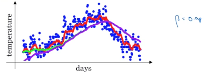
• Red is for \(\beta = 0.9\) with bias correction
• Green is for \(\beta = 0.98\) with bias correction
• Purple is for \(\beta = 0.98\) with**out** bias correction

\[\frac {v_t} {1-\beta^t}\]

As \(t\) increases the denominator will tend to 1.

Gradient descent with momentum

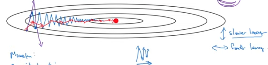
\[v_{dw} = \beta v_{dw} + (1-\beta) dw \\ v_{db} = \beta v_{db} + (1-\beta) db \\ w = w - \alpha \boxed{v_{dw}}\\ b = b - \alpha \boxed{v_{db}}\]

• Learning rate can be set to higher value with momentum.

RMSprop

when ever the gradient is changing drastically consistencly in a dimention its \(S_{dw^{[i]}}\) will be higher so dividing it by its square root will reduce its current gradient \(dw^{[i]}\) \[ S_{dw} = \beta S_{dw} + (1-\beta) dw^{\boxed{2}}\\ S_{db} = \beta S_{db} + (1-\beta) db^{\boxed{2}}\\ w = w - \alpha \frac {dw} {\boxed{\sqrt{S_{dw}}}}\\ b = b - \alpha \frac {db} {\boxed{\sqrt{S_{db}}}} \]

• Where \(dw^2\) is the elementwise square
• Here we are calling it as root mean square prop since we are squaring the derivatives and dividing the gradient by squreroot of the exponental weighted average of the gradient \(S^{dw}\).

Side note;

• The \(\beta\) here is not the same as momentum’s parameter.
• The \(\sqrt{S_{dw}}\) is added with \(\epsilon = 10^{-8}\) a small value to ensure the denomenator doesn’t go too close to zeoro.

Adam optimization

Adaptive moment estimation = RMSprop + Momentum

\[ v_{dw} = \beta_1 v_{dw} + (1-\beta_1) dw \\ v_{db} = \beta_1 v_{db} + (1-\beta_1) db \\ S_{dw} = \beta_2 S_{dw} + (1-\beta_2) dw^{2}\\ S_{db} = \beta_2 S_{db} + (1-\beta_2) db^{2}\\ v_{dw}^{corrected} = \frac {v_{dw}} {(1-\beta^t)}\\ v_{db}^{corrected} = \frac {v_{db}} {(1-\beta^t)}\\ S_{dw}^{corrected} = \frac {S_{dw}} {(1-\beta^t)}\\ S_{db}^{corrected} = \frac {S_{db}} {(1-\beta^t)}\\ w = w - \alpha \boxed{\frac {V_{dw}^{corrected}} {\sqrt{S_{dw}^{corrected}} + \epsilon}}\\ b = b - \alpha \boxed{\frac {V_{db}^{corrected}} {\sqrt{S_{db}^{corrected}} + \epsilon}} \]

Side note; On the original adam paper the following hyperparameter was used.

• \(\alpha\) needs to be tuned.
• \(\beta_1\) is 0.9.
• \(\beta_2\) is 0.999.
• \(\epsilon\) is \(10^{-8}\).

Learning rate decay

• \(\alpha = \frac 1 {{1 + decay\_rate * epoch\_number}} \alpha_{0}\)

• Exponentially decaying \(\alpha = 0.95^{epoch\_number} \alpha_{0}\)

• \(\alpha = \frac K {\sqrt{epoch\_number}} \alpha_{0}\)

• \(\alpha = 0.95^{t} \alpha_{0}\)

• Discreate starecase; after contant epoch reduce the learning rate by half.

If the model is training for days manually decay the learning rate.

1
2
3
4
5
6
7

a = 0.2 # learning rate a.
decay_rate = 1
number_of_epoch = 10

for epoch_number in range(1, number_of_epoch+1):
    a_decay = a / (1 + (decay_rate*epoch_number))
    print(f"Epoch {epoch_number}, Learning rate is {a_decay:5f}")

Batch normalization

Similar to normalizing the input with Preprocessing, this will normalize the intermidate outputs \(z^{[l]}\) of any layer (making the learning more efficient; ie trains W,b faster)

\[ \mu = \frac 1 {m} \sum_{i}^m z^{(i)} \\ \sigma^2 = \frac 1 {m} \sum_{i}^m ({z^{(i)}- \mu})**2\\ Z^{(i)}_{norm} = \frac {z - \mu} {\sqrt {\sigma^2}} \]

\(\tilde{Z}^{(i)} = \gamma Z^{(i)}_{norm} + \beta\)

Here

1. \(\beta\) is the mean \(\mu\).
2. \(\gamma\) is the standard deviation \(\sqrt{\sigma^2 +\epsilon}\).
3. The bias \(b\) is not required since in \(z_{norm}\) mean (\(\mu\)) subtraction will offsets \(b\).

\(\beta\), \(\gamma\) are both learnable parameter. Below gradient decent is used, althought Adam, RMSprop, or momentum can be used aswell. \[ \beta = \beta - \alpha \frac {dj} {d\beta}\\ \gamma = \gamma - \alpha \frac {dj} {d\gamma} \] Standard unit variance = variance =1

• Covariants shift is when the underlying training distribution is different from the testing environment. Batch norm, has a normalized input distribution reducing the noise added from weight updates from the previous layers.

• Slight regularization effect: As the batch norm is calculated on a minibatch, the mean and variance with which \(z_{norm}\) is scaled will add noise similar to the dropout adding noise to hidden layer’s activations.

  • Although its recommended to used dropout along with batch norm to do regularization.
  • More the batch size less the regularization.

At test time

\(\mu\) and \(\sigma^2\) is estimated using exponentially weighted average during training, similar to gradient with momentum and used during test time.