- https://www.youtube.com/watch?v=_i3aqgKVNQI&list=PLkDaE6sCZn6F6wUI9tvS_Gw1vaFAx6rd6
- https://towardsdatascience.com/introduction-to-word-embedding-and-word2vec-652d0c2060fa
- https://analyticsindiamag.com/word2vec-vs-glove-a-comparative-guide-to-word-embedding-techniques/
- https://towardsdatascience.com/word-embedding-techniques-word2vec-and-tf-idf-explained-c5d02e34d08
N-gram
n pairs of words in sentence.
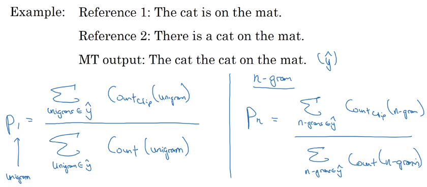
Bleu
Bilingual evaluation understudy
\[ bleu\ score = \frac {max\ number\ of\ occurances\ in\ reference} {total\ unique\ ngram} \]
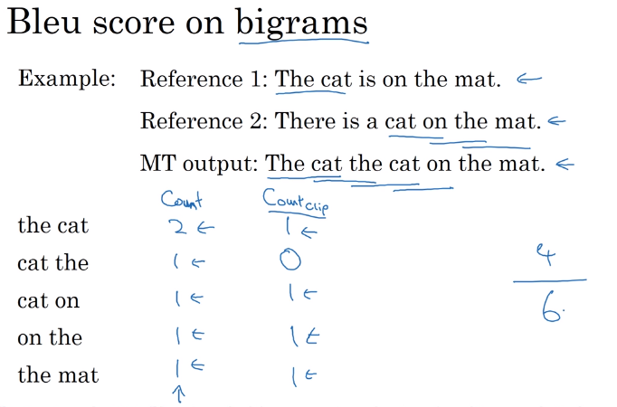
On uni and n grams
RNN
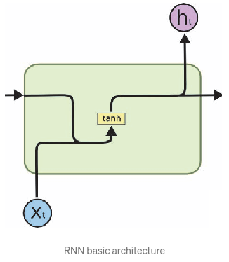
\[ h_t = tanh(W_{hs} h_{t-1} + W_{x} x_t) \]
The hidden state \(h_t\) is constantly rewritten at every time step causing to vanishing gradient over time. This makes the network not learn from dependencies from a longer time period.
To overcome this issue 2 types of RNN was developed.
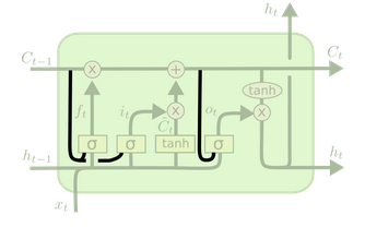
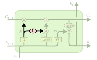
LSTM (Long Short Term Memory)
Gate
Remove or Add information from the cell state.
- Cell state \(C_t\)
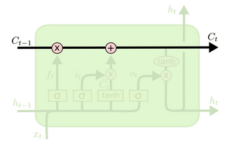
- Forget gate layer (What info to remove in cell state)
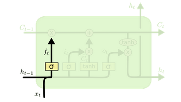
\(f_t = \sigma(W_f . [h_{t-1}, x_t] + b_f)\)
- Output 0,1 (for each number in the cell state \(C_{t-1}\))
- Input gate (What info to store in cell state)
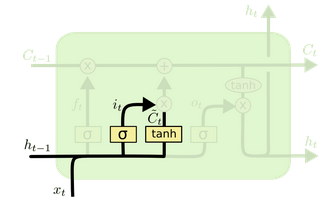
3.1) \(i_t = \sigma(W_i . [h_{t-1}, x_t]+ b_i)\) decides which input shall pass
3.2) \(\tilde{C} = tanh(W_c . [h_{t-1}, x_t]+ b_c)\) creates vector for cell state to be added into.
- Update the cell state
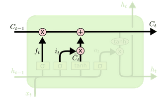
\[ C_{t} = f_t * C_{t-1} + i_t * \tilde{C} \]
- Output
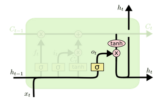
\[ o_t = \sigma(W_o . [h_{t-1}, x_t] + b_o)\\ h_t = o_t * tanh(C_t) \]
Variants of LSTM
- Adds peepholes (context for the gates on the current cell state \(C_t\)).
\[ f_t = \sigma(W_f . [\boxed{C_t}, h_{t-1}, x_t] + b_f)\\ i_t = \sigma(W_i . [\boxed{C_t}, h_{t-1}, x_t]+ b_i) \\ o_t = \sigma(W_o . [\boxed{C_t}, h_{t-1}, x_t] + b_o)\\ \]
- Coupled input and forget gates
\[ C_t = f_t * C_{t-1} + \boxed{(1-f_t)} * \tilde{C} \]
GRU (Gated Recurrent Unit)
GRU (Gated Recurrent Unit)
Merge forget and Input gate
Cell state and Hidden state.
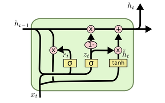
\[ z_t = \sigma(W_z . [h_{t-1}, x_t]) \\ r_t = \sigma(W_r . [h_{t-1}, x_t])\\ \tilde{h}_t = tanh(W . [r_t * h_{t-1}, x_t])\\ h_t = (1-z_t) * h_{t-1} + z_t * \tilde{h_t} \]
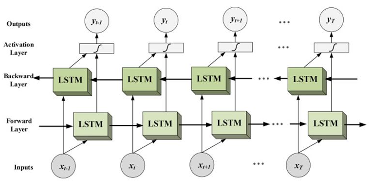
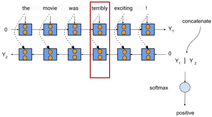
- BiLSTM
- Reference
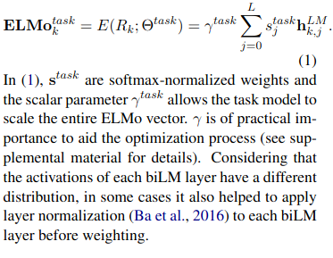
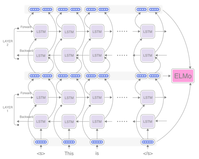
TODO Embeddings from language models (EL-mo)
or
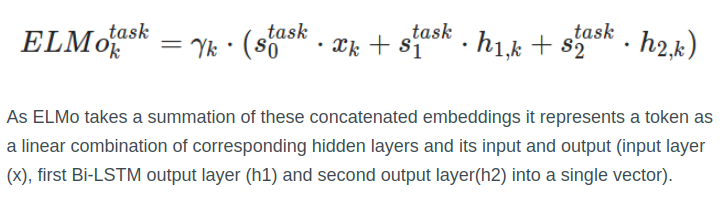
- word representations are from entire input sentence.
- predicts the next char from inputs seen so far.
- cost funtion: maximizes log likelihood of forward and backward prediction.
Note;
use this
or
- Reference
https://paperswithcode.com/method/elmo https://arxiv.org/pdf/1802.05365v2.pdf https://iq.opengenus.org/elmo/ https://indicodata.ai/blog/how-does-the-elmo-machine-learning-model-work/
Attention
Attention \(\alpha\) is weighted sum of activation ouput;
where \(\sum_{\grave{t}} \alpha^{<1,\grave{t}>} = 1\) (ofcouse with softmax :P) and the context \(C = \sum_{\grave{t}} \alpha^{<1,\grave{t}>} a^{<\grave{t}>}\)
Here \(a^{\grave{t}}\) is the activation from bidirectional rnn (from both the forward and backward).
the attention is computed with
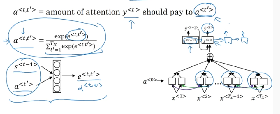
\[ e^<t,{\grave{t}}> = W \]
Time complexity is \(t_x t_y\) where \(t_x\) is the input length and \(t_y\) the output time length. Since for every output prediction we are calculating the attention \(\alpha\) for every input to generate the context \(C\).
https://arxiv.org/pdf/1502.03044v2.pdf
Transformers
https://www.tensorflow.org/text/tutorials/transformer http://jalammar.github.io/illustrated-transformer/
Bert model
Similar to ELmo, Bert also provides a contextual representation of the word embedding, but looks at the sentence all at once (with out having to concatenate forward and backward contextural hidden state vectors).
https://medium.com/analytics-vidhya/understanding-the-bert-model-a04e1c7933a9 https://www.youtube.com/watch?v=xI0HHN5XKDo
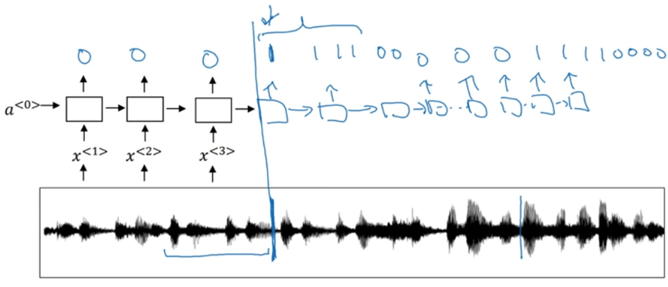
Audio data
Preprocessed to get the spectrogram (a visual representation of audio).
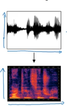
x axis time y axis small change in air pressure.
- when the input length is higher than output length
- A simple trigger word detection model.